In process engineering, heat capacity is an important property that determines
the amount of energy to provide to a system to raise its temperature.
However, there is not yet a group contribution approach that allows prediction
of heat capacity with temperature. The variations of heat capacity
with temperature are influenced by the quantification of the vibrational energy levels
[2][3]. This is probably why empirical
approaches are subject to difficulties. In the ideal gas state, these variations
can be reliably predicted by quantum chemistry methods [4]. In the
liquid or dense gas state, the prediction is a combination of an ideal contribution and
a residual contribution [5]:
\(C_{p}(T,P) = C_{p,id}(T) + C_{p,res}(T,P)\),
where the ideal gas heat capacity \(C_{p,id}(T,P)\) is the main term
containing vibrational, transitional, and rotational contributions, and the residual
term \(C_{p,res}(T,P)\) is predicted using classical statistical mechanics
or equations of state [6].
The present application note illustrates the high throughput capabilities of MedeA[1]
to predict ideal heat capacity of a substantial list of amides and alkanol amines
in a large temperature range (200-1,000 K). The results are then used to parametrize
a new functional form for \(C_{p,id}(T,P)\) allowing fast prediction and improved
physical relevance for engineering applications. For instance, the new functional
form is consistent with the continuously increasing trend of \(C_{p,id}(T,P)\)
and has the expected asymptotic limit. An original QSPR approach is developed to parametrize
the new expression.
34.2. Method and protocol
The list of compounds is assembled by retrieving SMILES strings from internet sources, namely,
Wikipedia, NIH, and NIST. A structure list is then created in MedeA by reading
a text file of names and SMILES strings. In order to sample the possible shapes, the
structure list contains up to ten stable conformers per compound, which are built by
exploring different sequences of dihedral torsion angles. Each conformer of the list
is structurally optimized using MedeA MOPAC with the semi-empirical PM7 method and
a vibrational analysis is performed.
The heat capacity is computed and printed for a list of regularly spaced temperatures
gathered in a property table in the Job.out file of the task, together with the enthalpy of
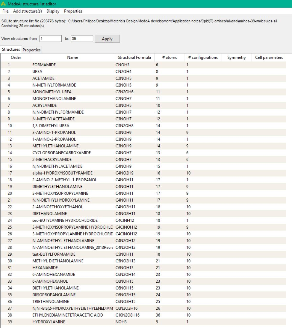
formation and entropy. The structure list comprises 36 species (Figure 34.2.1).
For each molecule, the lower energy
conformer is identified and its vibrational analysis is checked for the absence of
imaginary vibration frequencies. A corresponding property table is printed out for each species and
used to develop new QM-based correlations or compare with existing correlations
(for instance those from DIPPR).
Figure 34.2.1 Names and formulas for the training set of 36 compounds.
In the present work, we use the following functional form for \(C_{p,id}(T,P)\):
(34.2.1)\[C_{p,id}(T) = A + B \left[ \dfrac{\dfrac{C}{T}}{sinh(\dfrac{C}{T})} \right] ^{2} +
D \left[ \dfrac{\dfrac{E}{T}}{sinh(\dfrac{E}{T})} \right] ^{2}\]
where A, B, C, D, and E are theory-derived or empirical parameters.
If we set \(\theta_{\nu 1} = 2C\) and \(\theta_{\nu 2} = 2E\),
the above equation is exactly equivalent to the heat capacity of an ideal gas
of polyatomic molecules with two characteristic vibrational temperatures
\(\theta_{\nu 1}\) and \(\theta_{\nu 2}\)[2]. The
parameter B or D is the degeneracy (i.e. the weight) of each
vibrational frequency. The parameter A is the ideal heat capacity in the limit of low
temperature (translational + rotational contributions):
(34.2.2)\[A = R \left( \dfrac{5}{2} + \dfrac{p}{2} \right)\]
The number of rotational degrees of freedom is p = 2 for a linear molecule and p = 3
for a non-linear molecule. Another constraint is the asymptotic value in the limit of
high temperatures, which corresponds to a contribution of R/2 per vibrational degree
of freedom (in application of the equipartition of energy):
(34.2.3)\[B + D = R(3n-3-p)\]
where n is the total number of atoms. The model outlined in Equations
(34.2.1) - (34.2.3) has certainly
important limitations, e.g., it does not account for possible conformational changes, although it
maintains a low number of independent parameters (three), thus making their regression more
reliable. It is also ensuring a safe behavior in the low and high temperature limits. It may
be noted that Equation (34.2.1) is close from the equation used in DIPPR to correlate
\(C_{p,id}(T,P)\), the only difference being that DIPPR contains a term \(cosh(E/T)\)
instead of \(sinh(E/T)\). This may lead to some artifacts at high temperature
(see Appendix for more details and references about this equation).
34.3. Results
A standard flowchart of MedeAMOPAC for thermodynamic property prediction is
applied to the structure list of 39 amines and amides of
Figure 34.2.1, which contain 0 to 20 carbon atoms.
The list includes primary, secondary, tertiary, and quaternary cyclic or branched
amines and amides.
MedeA MOPAC helped finding ground state structure for each molecule, with the exception of
one hydrochlorinated amine which would require an improved initialization. The training
set contains 38 compounds, including two hydrochlorinated amines.
Thermodynamic properties are printed for temperatures between 308 and 808 K with a value each
10 K.
In a first step, the optimization for the parameters B, C, D, and E
is done separately for each compound.
The parameter A = 33.26 J mol-1 K-1
is identical for all compounds, as the set contains non-linear molecules exclusively.
B and D parameters increase with molecular size, as expected. The parameter C ranges
between 300 and 500 K, while most compounds exhibit values between 300 and 400 K. The parameter
E ranges from 1150 to 1450 K. These values correspond to \(\theta _{\nu 1} = 2C\) between 600 and 1000 K, and
\(\theta _{\nu 2} = 2E\) between 2300 and 2900 K, i.e., within the expected range of characteristic
vibrational temperatures.
In a second step, we correlate parameters A, B, C, D, and E with selected descriptors.
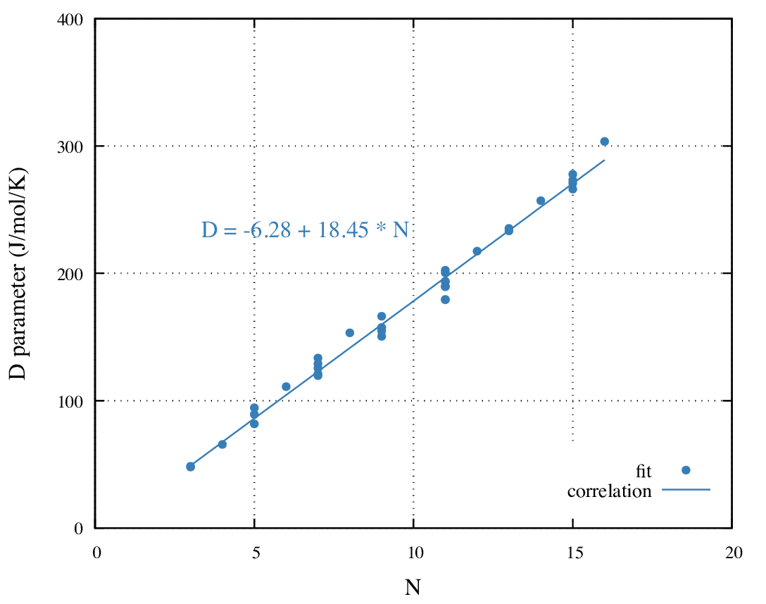
In Figure 34.3.1, the parameter B appears to vary linearly with the
total number of atoms with a regression coefficient of 0.97.
Figure 34.3.1 Variation of parameter B of Equation (34.2.1) with the total number of atoms
for the 36 amines of Figure 34.2.1.
The parameter D correlates best with the number of hydrogen atoms
nH (Figure 34.3.2). The regression coefficient is 0.99.
Figure 34.3.2 Variation of parameter D of Equation (34.2.1) with the number
of hydrogen atoms for the 36 amines of Figure 34.2.1.
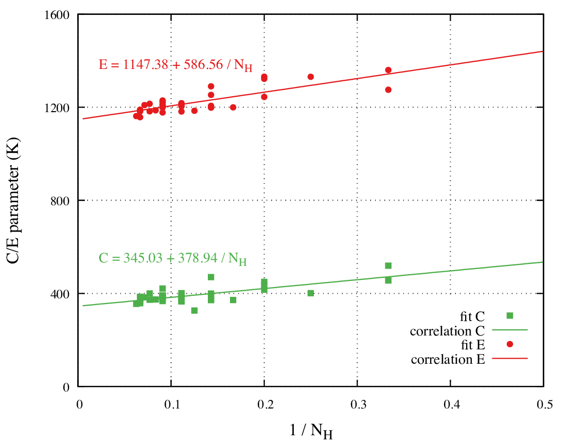
The parameters C and E also vary regularly, yet they
change faster for small carbon numbers. They correlate linearly
with \(\dfrac{1}{n_{H}}\) (Figure 34.3.3).
Figure 34.3.3 Variation of parameters C and E of Equation (34.2.1) with
the inverse number of hydrogen atoms.
The functional forms suggested by Figures 34.3.1 and
34.3.3 are:
(34.3.1)\[B = B_{0} + B_{1} \cdot n\]
(34.3.2)\[C = C_{0} + \dfrac{C_{1}}{n_{H}}\]
(34.3.3)\[D = D_{0} + D_{1} \cdot n_{H}\]
(34.3.4)\[E = E_{0} + \dfrac{E_{1}}{n_{H}}\]
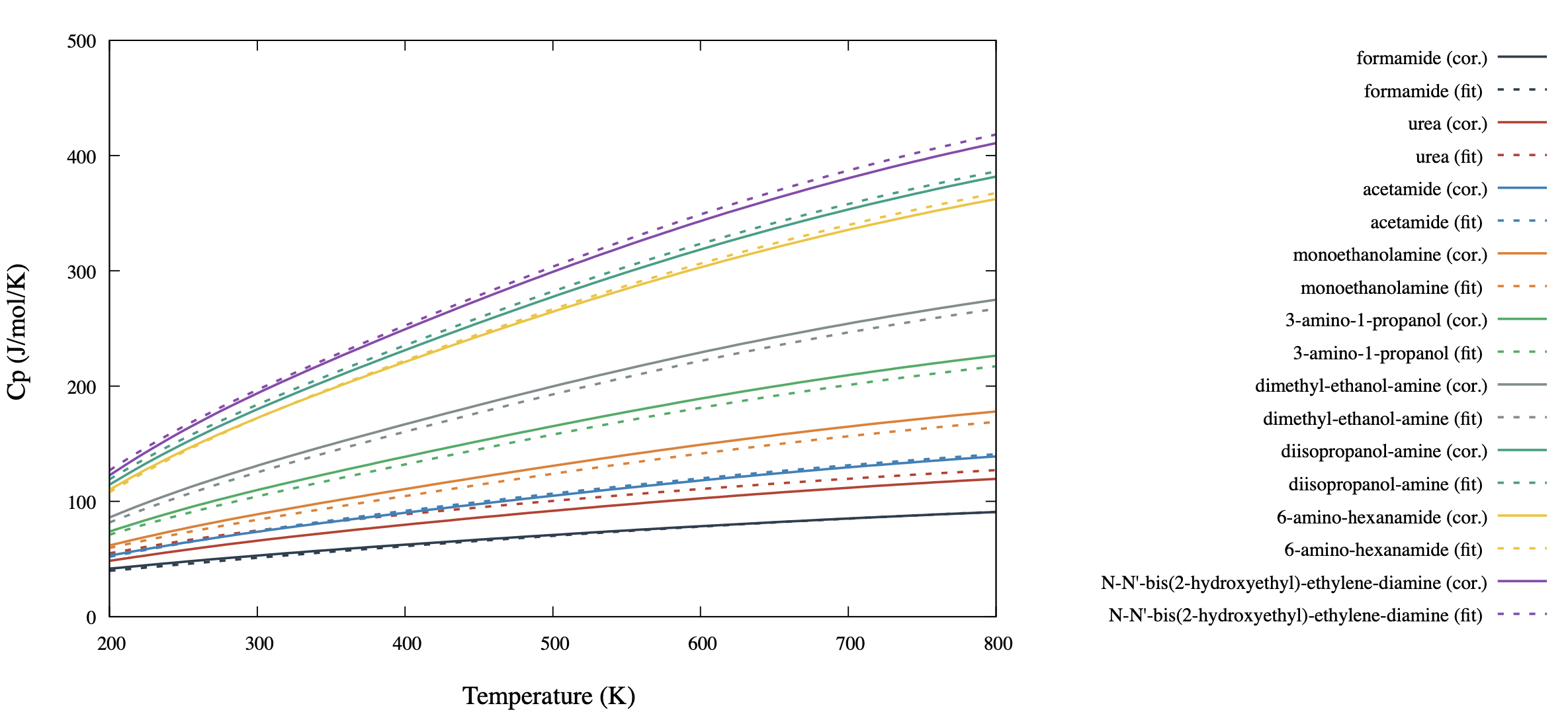
An outline of results is
indicated for a few selected compounds in (Figure 34.3.4).
Figure 34.3.4 Selected results of ideal gas heat capacity prediction for
alkanol amines and amides belonging to the training set of 36 molecules.
34.4. Conclusions
The proposed functional form involving two vibrational frequencies
(Equation (34.2.1)) allows parametrization from QM results covering the
relevant range for most engineering applications (308-808 K). The main
advantages are:
(i) each parameter has a physical meaning given by
quantum mechanics, ensuring consistent extrapolation to high
and low temperatures,
(ii) the stable optimization protocol
involves only three parameters per pure compound, hence not resulting in additional
computation cost for the end-user compared with DIPPR equations,
(iii) the regressed parameters vary regularly in homogeneous series, allowing to
build predictive correlations for \(C_{p,id}(T,n_{C})\), and
(iv) the approach can be extended to ideal gas energy and entropy with
theoretical expressions from [2].
The proposed methodology presents a substantial improvement compared
with previous methods (e.g. Benson’s method), which are not based on
explicit QM calculations with vibrational analysis. It is also a
substantial progress compared to experiment-based correlation work (e.g.
DIPPR project, Poling’s textbook [7]), which predict sometimes
unrealistic \(C_{p,id}(T)\) at high temperature. Further
improvement is still possible by increasing the number of parameters,
for instance, introducing a third vibration frequency in Equation
(34.2.1) or additional descriptors, or adding the effect of
possible chemical transformations or conformational changes, and testing
correlations with an independent validation dataset.
Appendix
The equation provided by Mc Quarrie (1976) for a polyatomic gas is:
where k is the Boltzmann constant, N is the Avogadro number. The number of
rotational degrees of freedom is p = 2 for a linear molecule and
p = 3 for a non-linear molecule. The index j runs over the
vibrational degrees of freedom, and \(\vartheta_{\text{vj}}\) is the
characteristic vibrational temperature associated with the
jth vibrational degree of freedom.
If we introduce \(C_{j} = \ \frac{\vartheta_{\text{vj}}}{2}\),
considering that \(C_{p,id}-C_{v,id} = R = N*k\) for an ideal gas,
Equation (34.4.1) rearranges into:
If the summation is simplified assuming two frequencies, we obtain
Equation (34.2.1). We can compare it with the Equation that
correlates with the ideal heat capacity, \(C_{p,id}(T)\) in DIPPR:
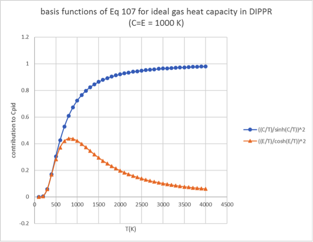
(34.4.3)\[C_{p,id} = A + B \bullet \left\lbrack \frac{\frac{C}{T}}{\sinh\left( \frac{C}{T} \right)} \right\rbrack^{2} + D \bullet \left\lbrack \frac{\frac{E}{T}}{\cosh\left( \frac{E}{T} \right)} \right\rbrack^{2}\]
is not. A more detailed analysis shows a decrease of the vibrational
contribution when temperature increases up to several thousand K.
Figure 34.4.1 Comparison of the two terms
\(\left\lbrack \frac{\frac{C}{T}}{\sinh\left( \frac{C}{T} \right)} \right\rbrack^{2}\)
and
\(\left\lbrack \frac{\frac{E}{T}}{\cosh\left( \frac{E}{T} \right)} \right\rbrack^{2}\)
with temperature in Equation (34.2.1). The constants C and E are set to
1000 K in this example.