5. Structural Properties & Surface Area of Clay Minerals

In this note, we illustrate the predictive power of MedeA^®[1] for characterizing clay minerals by means of forcefield based Molecular Dynamics and Grand Canonical Monte Carlo.

Keywords: clays, clay minerals, forcefield, physisorption, BET, surface area, GCMC

5.1. Introduction

Clay minerals are widely encountered in industrial processes ranging from ceramics manufacturing, oil exploration and production, nuclear waste storage to management of water resources and civil engineering or soil science.

Given the small size of clay particles and their rather complex chemistry, classical analytical techniques, such as XRD, are not able to provide a complete model of the clay structure at the nanoscale. Therefore, molecular modeling is useful to complement classical analysis in studying possible structure variations in a given family, as a result of cation location, amount of interstitial water, etc. Moreover, molecular models can also help in understanding property/structure relations.

In this note, we compare computed structural properties of clay minerals with experimental data, wherever such data is available. Calculated properties include cell parameters, atomic positions (in particular H positions) and internal surface areas. The assessment of the interactions of clay minerals with fluids (thereby influencing adsorption capacity, swelling, cation exchange and diffusivity) is subject to a separate application note.

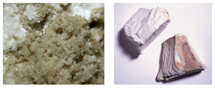
Figure 5.1.1 Left: Boehmite and Natrolite from Sagåsen (Strandåsen), Mørje, Porsgrunn, Telemark, Norway [2] (Field of view 10 mm); Right: Kaolinite [3].

5.2. Molecular Modeling

The initial structures used here are obtained from the Inorganic Crystal Structure Database (MedeA InfoMaticA) (Boehmite, Portandlite, Kaolinite and Pyrophyllite).

To begin with, we employ molecular dynamics (MD) simulations as implemented in MedeA LAMMPS to relax atomic positions and cell parameters of bulk clay minerals and clay pores. To do so, we run subsequent NVT and NPT ensembles calculations of a duration of 100-200 ps for each ensemble.

The resulting structures are then subjected to Grand Canonical Monte Carlo (GCMC) simulations (MedeA GIBBS), where simulated BET [4] analysis is performed to determine the specific surface area of the clay pore(s).

Table 5.2.1 Methods for determining clay mineral properties from experiment and molecular simulation

Property	Experimental Method	Simulation Method
Unit Cell Parameters	Diffraction	Energy minimization, MD NPT simulation
Local Atomic Coordination	EXAFS, Structure Factor	Radial Distribution Fucntion from MD and/or MC simulation
Mechanical Properties	Nanoidentation	Energy minimization, MD simulation
Surface Area	N2BET at 77K	N2BET at 77K, GCMC simulation

The CLAYFF forcefield [5] is used to describe the clays in both MD and MC simulations. For nitrogen, a molecular model with two force centers on the nitrogen atoms and three charges is being used [6].

5.3. Results

Boehmite [AlO(OH] and Portlandite [Ca(OH)₂] are two minerals composed of octahedral layers (O). Kaolinite [Al₂Si₂O₅(OH)₄] and Pyrophyllite [AlSi₂O₅(OH)₂] are two clay minerals respectively composed of tetrahedral (T) and octahedral (O) layers (specifically: TO and TOT) (Figure 5.3.1).

The hydrogen position is generally undetermined in the crystallographic data. Therefore, hydrogen atoms are initially positioned according to general observations and chemistry constraints and their final position is obtained from the resulting configurations of the MD simulations.

Cell parameters, angles and densities are obtained by NPT simulations and compare well to published experimental data (Table 5.3.1, Table 5.3.2, Table 5.3.3 and Table 5.3.4).

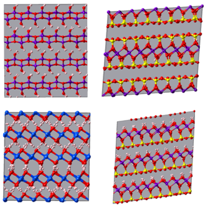
Figure 5.3.1 Clay mineral structures simulated with CLAYFF (NPT simulation for 100 ps, 300 K, 1 bar). Top Left: Boehmite, Top Right: Kaolinite, Bottom Left: Portlandite and Bottom Right: Pyrophyllite. Atom color code: O (red), H (white), Al (purple), Si (yellow) and Ca (blue).

Table 5.3.1 Comparison of structural properties of Boehmite from Molecular Dynamics (NPT Simulations at 300 K, 1 bar for 100 ps) and experiment.

Boehmite AlO(OH)	Exp. [7]	Cygan et al. [5]	MedeA LAMMPS
a (|AA|)	2.9	3.0	3.0
b (|AA|)	12.2	12.4	12.4
c (|AA|)	3.7	3.7	3.7
\(\alpha\) (\(^{ \circ}\))	90	90	90
\(\beta\) (\(^{ \circ}\))	90	90	90
\(\gamma\) (\(^{ \circ}\))	90	90	90
\(\rho\) (g/ml)	3.05	2.88	2.94

Table 5.3.2 Cell Parameters, Comparison of structural properties of Portlandite Ca(OH)₂ from Molecular Dynamics (NPT Simulations at 300 K, 1 bar for 100 ps) and experiment.

Portlandite Ca(OH)2	Exp. [8]	Cygan et al. [5]	MedeA LAMMPS
a (\({\mathring{\mathrm{A}}}\))	3.6	3.7	3.5
b (\({\mathring{\mathrm{A}}}\))	3.6	3.7	3.5
c (\({\mathring{\mathrm{A}}}\))	4.9	4.8	4.7
\(\alpha\) (\(^{ \circ}\))	90	82	92
\(\beta\) (\(^{ \circ}\))	90	98	89
\(\gamma\) (\(^{ \circ}\))	120	122	120
\(\rho\) (g/ml)	2.25	2.24	2.47

Table 5.3.3 Comparison of structural properties of Kaolinite from Molecular Dynamics (NPT Simulations at 300 K, 1 bar for 100 ps) and experiment.

Kaolinite	Exp. [9]	Cygan et al. [5]	MedeA LAMMPS
a (\({\mathring{\mathrm{A}}}\))	5.2	5.2	5.2
b (\({\mathring{\mathrm{A}}}\))	8.9	9.0	8.9
c (\({\mathring{\mathrm{A}}}\))	7.4	7.4	7.3
\(\alpha\) (\(^{ \circ}\))	92	91	90
\(\beta\) (\(^{ \circ}\))	105	104	100
\(\gamma\) (\(^{ \circ}\))	90	90	90
\(\rho\) (g/ml)	2.61	2.58	2.77

Table 5.3.4 Comparison of structural properties of Pyrophyllite from Molecular Dynamics (NPT Simulations at 300 K, 1 bar for 100 ps) and experiment.

Pyrophyllite	Exp. [10]	Cygan et al. [5]	MedeA LAMMPS
a (\({\mathring{\mathrm{A}}}\))	5.2	5.2	5.2
b (\({\mathring{\mathrm{A}}}\))	9.0	9.0	9.0
c (\({\mathring{\mathrm{A}}}\))	9.3	9.5	9.3
\(\alpha\) (\(^{ \circ}\))	91	91	90
\(\beta\) (\(^{ \circ}\))	100	99	98
\(\gamma\) (\(^{ \circ}\))	90	90	90
\(\rho\) (g/ml)	2.82	2.74	2.77

The specific surface area is calculated using the BET equation (5.3.1):

(5.3.1)\[\frac{p}{n_{a}\ (p_{0} - p)} = \frac{1}{n_{m}C} + \frac{\left( C - 1 \right)}{n_{m}C}.\frac{p}{p_{0}}\]

where \(n_{a}\) is the sorbed amount of N₂, \(\frac{p}{p_{0}}\) is the relative pressure and \(n_{m}\) is the monolayer capacity of N₂ per simulation box.

Plotting \(\frac{p}{n_{a\ (p_{0} - p)}} = f(\frac{p}{p_{0}})\) permits us to calculate \(n_{m}\) and therefore the surface area, A_(BET):

(5.3.2)\[A_{(BET)} = n_{m} a_{m}\]

where \(a_{m}\) is the molecular cross-sectional area of the N₂ molecules equals to 0.162 nm² at 77 K (Figure 5.3.2). The surface of pyrophyllite per simulation box, A_(BET), is equal to 17.21 nm², which for our system gives a specific surface area of 13.7 m²/g of clay (our system contains 7 layers and a pore width ~3.5 nm).

At low relative pressure, nitrogen forms one layer on clay surface. As pressure increases, a second nitrogen layer is formed. Further increase of the pressure leads to multilayer formation and finally filling of the pore with liquid nitrogen at pressures near the saturation pressure of nitrogen.

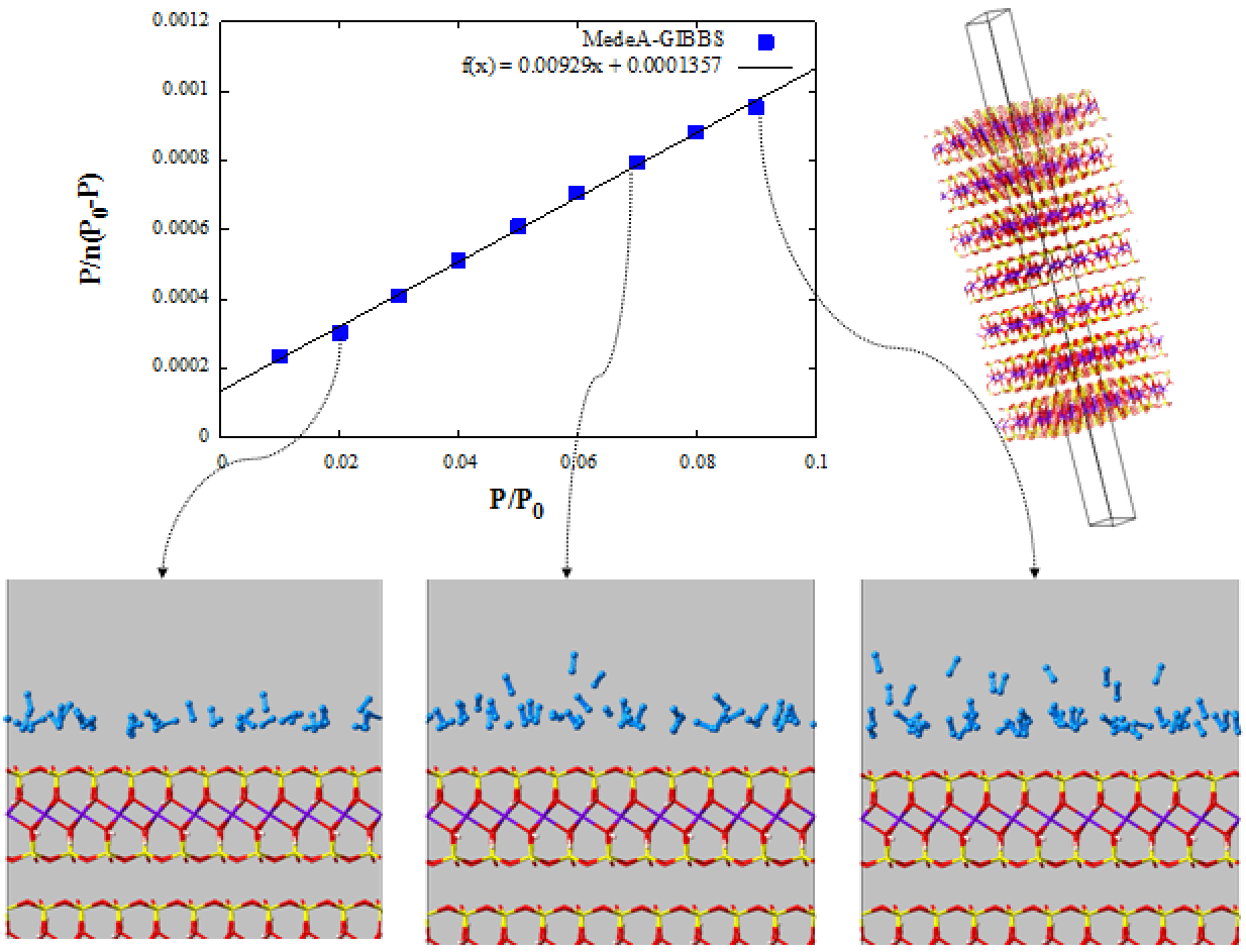
Figure 5.3.2 BET graph & Snapshots of nitrogen adsorption on pyrophyllite at 77 K and different relative pressure (0.02 on the bottom left, 0.07 in the middle and 0.09 on the right). Only part of the simulation box is shown, with part of the solid and part of the pore. Atom color code: O (red), H (white), Al (purple), Mg (green) Si (yellow), N (light blue).

5.4. Conclusions

We have demonstrated the ability to use forcefield simulations (Molecular Dynamics and Monte Carlo) to describe clay minerals both in bulk form and when forming nanopores. Here, we examine the properties of a pore of a fixed size and shape and its formation is not part of this note but clay swelling and relevant phenomena are addressed in another application note.

Characterization of such systems can be performed by means of molecular simulation, reproducing the experimental methods that are largely used for this purpose, such as BET surface area calculation with nitrogen adsorption at 77 K.

In the simple pore geometry used in this note, the surface area is actually input of the model and this example serves only as a demonstration of how a surface area calculation takes place, which is essential for more complex geometries, where a simple geometric determination is not an option.

Characterization of such systems is the first step and a very important one in the study of more complex phenomena like the adsorption and diffusion of organic mixtures in the presence of water or inorganic compounds, like CO₂, in pores of different sizes and geometries.

[1]

MedeA and Materials Design are registered trademarks of Materials Design, Inc.

[2]

“Böhmite-89904” by Leon Hupperichs source: (link)

[3]

“KaoliniteUSGOV”, source: (link)

[4]

Y. S. Bae et al., “Evaluation of the BET Method for Determining Surface Areas of MOFs and Zeolites that Contain Ultra-Micropores”, Langmuir 26, 5475 (2010) (link)

[5] (1,2,3,4,5)

R. T. Cygan et al., “Molecular Models of Hydroxide, Oxyhydroxide, and Clay Phases and the Development of a General Force Field”, J. Phys. Chem. B 108, 1255 (2004) (link)

[6]

J. Delhommelle, PhD thesis, Universite de Paris XI, Orsay, France, (2000)

[7]

A. N. Christensen et al., “Deuteration of Crystalline Hydroxides. Hydrogen Bonds of gamma-AlOO(H,D) and gamma-FeOO(H,D)”, Acta Chem. Scand. 36, 303 (1982) (link)

[8]

L. Desgranges et al., “Hydrogen thermal motion in calcium hydroxide: Ca(OH)₂", J. C. Acta Crystallogr. Sect. B, Struc. Sci. 49, 812 (1993) (link)

[9]

D. L. Bish, “Rietveld refinement of the kaolinite structure at 1.5 K”, Clays and Clay Minerals 41, 738 (1993) (link)

[10]

J. H. Lee et al., “Single crystal X-ray refinement of pyrophyllite-1 Tc”, Am. Mineral. 66, 350 (1981)

download:

pdf